stress_concentration

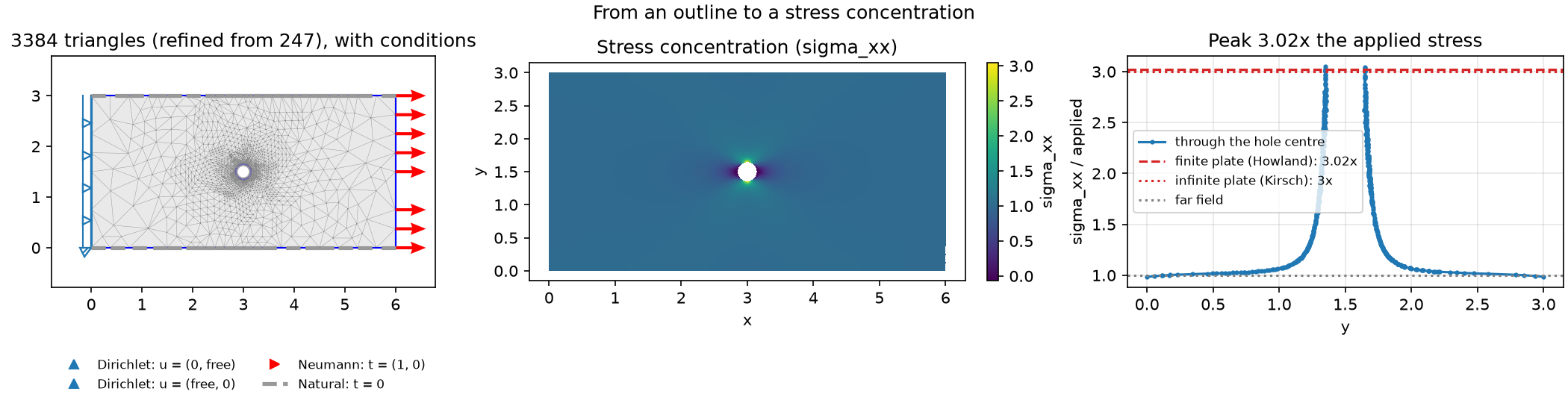
"""A plate with a hole, from outline to the stress concentration at its rim, against
Kirsch and Howland.

The one demo that runs the whole pipeline, so it builds its own mesh: the outline, what
Ruppert's was asked for, and where the conditions went are part of what it shows.
`mesh_plate`, `plate_bc`, and `refine_to_the_rim` each do one step; `run` calls them
and returns a `PlateStudy` of plain results. Nothing here draws: `figures.py` does
that from the `PlateStudy`, and this file is what the gallery shows.
"""
from dataclasses import dataclass

import numpy as np

from fem.analysis.adaptivity import AdaptiveRefinement
from fem.analysis.estimators import RecoveryEstimator
from fem.boundary import Dirichlet, Neumann
from fem.conditions import Conditions
from fem.elements import IsoparametricTriangleElement
from fem.mesh.curves import Circle
from fem.mesh.mesh import Mesh
from fem.mesh.outline import Outline
from fem.mesh.pslg import PSLG
from fem.physics.equations import LinearElastic
from fem.post.solution import ElasticSolution
from fem.regions import intersect, on_plane


def plate_with_hole_outline(length: float = 6.0, height: float = 3.0,
                            radius: float = 0.3) -> Outline:
    """A `length` x `height` plate with a circular hole at its centre.

    Two loops: the outline and the hole, which under the even-odd rule is a hole rather
    than a second region. The hole is a `Circle`, so refinement rounds it and an
    isoparametric solve places its boundary nodes on the true rim.
    """
    plate = np.array([[0.0, 0.0], [length, 0.0], [length, height], [0.0, height]])
    return Outline([Outline.from_polygons([plate]).loops[0],
                    Circle([length / 2, height / 2], radius)])

equation = LinearElastic(E=200, nu=0.3)


def finite_plate_kt(hole_over_width: float) -> float:
    """Howland's stress concentration factor for a circular hole in a finite-width plate
    under tension, relative to the applied (gross) stress. Peterson's polynomial fit
    gives the factor on the net section; dividing by the net fraction of width puts it
    on the applied stress. Reads Kirsch's 3 for a vanishing hole."""
    r = hole_over_width
    net = 3.000 - 3.140 * r + 3.667 * r**2 - 1.527 * r**3
    return net / (1.0 - r)


def rim_facets(mesh: Mesh) -> int:
    """How many boundary facets lie on the hole: `plate_with_hole_outline` draws the hole
    as loop 1, and Ruppert's tags every facet with the loop it came from."""
    assert mesh.boundary_tags is not None
    return int(np.sum(mesh.boundary_tags == 1))


def mesh_plate(length, height, radius, rim_chords, min_angle,
               max_area_fraction) -> tuple[PSLG, Mesh]:
    """The sampled outline and its coarse Ruppert's triangulation.

    The hole is sampled as a coarse `rim_chords`-gon, which is enough: the hole is a
    `Circle`, so Ruppert's split points, red-green refinement, and the isoparametric
    element's edge nodes all land on the true rim. The mesh's `boundary_tags` name the
    rim (loop 1) on every mesh refinement builds from it.
    """
    outline = plate_with_hole_outline(length, height, radius)
    graph = outline.sample(resolution=2 * np.pi * radius / rim_chords / outline.extent)
    # Coarse: resolving the rim is adaptive refinement's job. The rim still grades
    # finer than the interior, since Ruppert's honours its short segments.
    return graph, graph.mesh(min_angle=min_angle, max_area_fraction=max_area_fraction)


def plate_bc(length, traction) -> Conditions:
    """A roller on the left, tension on the right, and nothing on the rim.

    The rim takes no condition: a free surface is the natural boundary condition of
    the weak form, so "traction-free" is what an edge means when nothing is said.

    The left edge is a roller, not a clamp: pinned normal to itself (x = 0), free
    tangentially (y) so the plate can narrow as it stretches. A clamp would resist
    that Poisson contraction and add its own stress concentration, which competes with
    the hole for the estimator's attention. Pinning y along the edge would do the same,
    so a second condition pins y at one corner only, removing the last rigid-body mode.
    The conditions are written against coordinates, so they resolve against whatever
    triangulation arrives, including the ones adaptive refinement rebuilds.
    """
    return Conditions(
        Dirichlet(on_plane(0, 0.0), [0, None]),
        Dirichlet(intersect(on_plane(0, 0.0), on_plane(1, 0.0)), [None, 0]),
        Neumann(on_plane(0, length), [traction, 0]),
    )


def refine_to_the_rim(mesh: Mesh, bc: Conditions, refinement_iters,
                      refinement_budget) -> tuple[Mesh, ElasticSolution]:
    """Solve on the curved quadratic element, adaptively refined by the recovery
    estimator, which reads the curved rim's stress correctly.

    The rim splits project onto the true circle, so more refinement keeps rounding the
    hole. Everything measured afterwards is read off the refined mesh.
    """
    refinement = AdaptiveRefinement(
        mesh, lambda m: equation.problem(m, bc, element_type=IsoparametricTriangleElement),
        RecoveryEstimator(),
        max_triangles=len(mesh.elements) + refinement_budget, max_iters=refinement_iters,
    )
    solution = refinement.run()
    return refinement.mesh, solution


@dataclass
class PlateStudy:
    """Everything `run` computed, for the figures and the summary to read."""
    length: float
    height: float
    radius: float
    traction: float
    min_angle: float
    pslg: PSLG
    bc: Conditions
    n_initial: int                  # triangles before adaptive refinement
    initial_worst_angle: float
    initial_rim_facets: int
    mesh: Mesh                      # after refinement
    solution: ElasticSolution
    sigma_xx: np.ndarray            # nodal stress on the refined mesh
    y_strip: np.ndarray             # the strip through the hole centre, sorted by y
    ratio_strip: np.ndarray         # sigma_xx / traction along it
    peak: float                     # rim sigma_xx / traction

    @property
    def hole_over_width(self) -> float:
        return 2*self.radius / self.height

    @property
    def finite_kt(self) -> float:
        """Howland's finite-plate factor at this hole/width ratio."""
        return finite_plate_kt(self.hole_over_width)

    @property
    def worst_angle(self) -> float:
        """Ruppert's angle guarantee does not survive red-green refinement, which bisects
        existing triangles rather than re-triangulating for shape; reported rather than
        hidden."""
        return self.mesh.min_angle

    @property
    def rim_facets(self) -> int:
        """The rim facets of the refined mesh: the tag survives every split."""
        return rim_facets(self.mesh)


def run(traction=1.0, length=6.0, height=3.0, radius=0.15, min_angle=25,
        max_area_fraction=0.01, rim_chords=16, refinement_iters=36,
        refinement_budget=40000) -> PlateStudy:
    """Mesh the plate, refine into the rim, and read the concentration off it."""
    pslg, mesh = mesh_plate(length, height, radius, rim_chords, min_angle,
                            max_area_fraction)
    n_initial, initial_worst_angle = len(mesh.elements), mesh.min_angle
    initial_rim_facets = rim_facets(mesh)
    bc = plate_bc(length, traction)
    mesh, solution = refine_to_the_rim(mesh, bc, refinement_iters, refinement_budget)

    # The stress at the nodes: each element evaluated at its own nodes and averaged
    # where they meet, so the rim value is read on the rim itself.
    nodes = solution.space.node_coords
    sigma_xx = solution.nodal_stress()[:, 0, 0]

    # A vertical strip through the hole's centre: the line the concentration decays
    # along. The rim crossings are mesh nodes (the 16-gon has a vertex at the top and
    # bottom of the hole, and refinement keeps it), so the peak is the value there.
    strip = np.abs(nodes[:, 0] - length/2) < 0.25*radius
    order = np.argsort(nodes[strip, 1])
    y_strip, ratio_strip = nodes[strip, 1][order], (sigma_xx[strip] / traction)[order]
    on_rim = (np.isclose(nodes[:, 0], length/2)
              & np.isclose(np.abs(nodes[:, 1] - height/2), radius))
    peak = float(sigma_xx[on_rim].max() / traction)

    # Two reference values. Kirsch's factor of 3 is for a hole in an infinite plate.
    # This plate is finite, and the hole removes some of its section, so the remaining
    # material carries slightly more stress and the exact peak is a little above 3.
    # Howland (1930) worked out that finite-width correction for a strip with a central
    # hole; `finite_plate_kt` gives his value at this hole/width ratio, and that is the
    # line the measured peak is judged against.
    #
    # The peak converges to it from below, since a finite element solution is slightly
    # too stiff and the steepest gradient is the last thing it resolves: 2.97, 3.00,
    # 3.00, 3.03 over 624, 970, 1877 and 3301 elements. Thirty-six rounds is enough to
    # agree to within a hundredth.
    return PlateStudy(length, height, radius, traction, min_angle, pslg, bc,
                      n_initial, initial_worst_angle, initial_rim_facets, mesh, solution,
                      sigma_xx, y_strip, ratio_strip, peak)