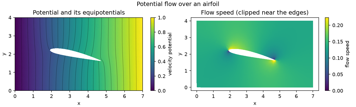
Poisson's equation as potential flow over a NACA airfoil, on P2 elements.
uv run python examples/cli.py run poisson
The functions that pose and solve the problem. The figures are below the fold.
"""Poisson's equation as potential flow over a NACA airfoil, on P2 elements.

`run` meshes the airfoil in its channel and solves Laplace's equation for the velocity
potential, returning a `FlowStudy` of plain results. Nothing here draws: `figures.py`
does that from the `FlowStudy`, and this file is what the gallery shows.
"""
from dataclasses import dataclass

import numpy as np

from fem.boundary import Dirichlet
from fem.conditions import Conditions
from fem.elements import QuadraticTriangleElement
from fem.loads import Source
from fem.mesh.mesh import Mesh
from fem.mesh.outline import Outline
from fem.physics.equations import Poisson
from fem.post.solution import DiffusionSolution
from fem.regions import on_plane


def _naca4_outline(camber: float, camber_pos: float, thickness: float, n: int,
                   te_trim: float = 0.05) -> np.ndarray:
    """A NACA 4-digit airfoil as a closed loop of points, unit chord along +x.

    `camber` (m), `camber_pos` (p), and `thickness` (t) are the usual fractions: a NACA
    2412 is (0.02, 0.4, 0.12). Cosine node spacing clusters points at the leading and
    trailing edges, where the curvature is highest.

    `te_trim` cuts that fraction of the chord off the trailing edge, leaving a blunt
    edge in place of the near-cusp a full 4-digit section tapers to, which the mesher
    would chase with unboundedly many tiny triangles.
    """
    beta = np.linspace(0, np.pi, n)
    x = 0.5 * (1 - np.cos(beta)) * (1 - te_trim)    # cosine spacing, 0 (LE) to 1-te_trim (TE)
    yt = 5 * thickness * (0.2969 * np.sqrt(x) - 0.1260 * x - 0.3516 * x**2
                          + 0.2843 * x**3 - 0.1015 * x**4)
    if camber > 0 and 0 < camber_pos < 1:
        m, p = camber, camber_pos
        yc = np.where(x < p, m / p**2 * (2 * p * x - x**2),
                      m / (1 - p)**2 * ((1 - 2 * p) + 2 * p * x - x**2))
        dyc = np.where(x < p, 2 * m / p**2 * (p - x), 2 * m / (1 - p)**2 * (p - x))
    else:
        yc = dyc = np.zeros_like(x)                 # symmetric section (m = 0)
    theta = np.arctan(dyc)
    upper = np.column_stack([x - yt * np.sin(theta), yc + yt * np.cos(theta)])
    lower = np.column_stack([x + yt * np.sin(theta), yc - yt * np.cos(theta)])
    # Trailing edge over the top to the leading edge, then back under; the shared leading
    # edge is dropped so it is not duplicated.
    return np.vstack([upper[::-1], lower[1:]])


def airfoil_channel_outline(length: float = 7.0, height: float = 4.0, chord: float = 3.0,
                         angle_of_attack: float = 6.0, camber: float = 0.02,
                         camber_pos: float = 0.4, thickness: float = 0.12,
                            n_points: int = 100) -> Outline:
    """A rectangular channel with a NACA 4-digit airfoil obstacle in it.

    The airfoil is generated analytically (no data file needed), scaled to `chord`,
    pitched `angle_of_attack` degrees nose-up into a left-to-right flow, and placed in
    the channel. The default is a NACA 2412. Under the even-odd rule the airfoil loop is
    a hole, so a mesh covers the fluid and stops at the wing, making its surface a
    boundary the solver sees (and, taking no condition, a streamline).
    """
    foil = _naca4_outline(camber, camber_pos, thickness, n_points)
    foil = foil * chord - [0.35 * chord, 0.0]       # pivot near the quarter-chord
    a = np.deg2rad(angle_of_attack)
    c, s = np.cos(a), np.sin(a)
    foil = foil @ np.array([[c, -s], [s, c]])       # nose up into the +x flow
    foil = foil + [0.42 * length, 0.5 * height]
    channel = np.array([[0.0, 0.0], [length, 0.0], [length, height], [0.0, height]])
    return Outline.from_polygons([channel, foil])


@dataclass
class FlowStudy:
    """Everything `run` computed, for the figures to read."""
    angle_of_attack: float
    mesh: Mesh
    bc: Conditions
    solution: DiffusionSolution      # the velocity potential phi, on P2

    @property
    def speed(self) -> np.ndarray:
        """|v| = |grad(phi)|, read at the nodes so the P2 tessellation draws it smoothly."""
        return np.linalg.norm(self.solution.nodal_gradient(), axis=1)   # (n_nodes,)

    @property
    def speed_cap(self) -> float:
        """Ideal flow with no Kutta condition predicts a near-singular velocity at the
        sharp edges; clip it to a high percentile so the flow over the wing stays legible."""
        return float(np.percentile(self.speed, 96))


def run(length=7.0, height=4.0, chord=3.0, angle_of_attack=12.0, n_points=80, min_angle=20,
        max_area_fraction=0.0015) -> FlowStudy:
    """Mesh the airfoil in its channel and solve for the velocity potential."""
    # An ideal (incompressible, irrotational) flow has a velocity potential phi with
    # v = grad(phi) and div(v) = 0, so phi solves Laplace's equation, Poisson's with no
    # source. The wing carries no
    # flow through it, the natural (zero-flux) condition of the weak form: say nothing
    # on its surface and it becomes a streamline the flow parts around.
    outline = airfoil_channel_outline(length, height, chord, angle_of_attack, n_points=n_points)
    mesh = outline.mesh(min_angle=min_angle, max_area_fraction=max_area_fraction)

    equation = Poisson()   # Laplace: no sources in the flow
    # phi rises from inlet to outlet, so v = grad(phi) runs left to right. The wing and
    # the walls take no condition, so they are no-flux streamlines.
    bc = Conditions(
        Dirichlet(on_plane(0, 0.0), 0.0),
        Dirichlet(on_plane(0, length), 1.0),
    )

    problem = equation.problem(mesh, bc + Source(0), element_type=QuadraticTriangleElement)
    solution = problem.solve()
    return FlowStudy(angle_of_attack, mesh, bc, solution)
"""The figures of the airfoil potential-flow demo, drawn from a `FlowStudy`."""
from demo_registry import Demo, DemoResult, Figure

from demos._charts import conditions_figure
from demos.poisson import physics
from demos.poisson.physics import FlowStudy, run
from fem.plot.plotter import Plotter


def _flow_figure(s: FlowStudy) -> Figure:
    # `space=solution.space` opts both panels onto the P2 tessellation: the potential
    # shows its within-element curvature and the recovered speed draws smoothly.
    plotter = Plotter(1, 2, title='Potential flow over an airfoil', panel_aspect=1.8)
    plotter.plot(s.mesh, s.solution.dofs, mode='colored', idx=(0, 0), label='velocity potential',
                 title='Potential and its equipotentials', contour=22, space=s.solution.space)
    plotter.plot(s.mesh, s.speed, mode='colored', idx=(0, 1), label='flow speed',
                 clim=(0.0, s.speed_cap), title='Flow speed (clipped near the edges)',
                 space=s.solution.space)
    return Figure(
        plotter,
        'Ideal (irrotational, incompressible) flow over a NACA 2412 airfoil at a '
        f'{s.angle_of_attack:g}-degree angle of attack, generated from the standard '
        'formula rather than a data file. Left: the velocity potential phi (Laplace) '
        'with its equipotentials, which crowd over the upper surface where the flow '
        'speeds up. Right: the flow speed, faster over the top than the bottom, with '
        'stagnation near the leading and trailing edges. The wing takes no condition '
        'at all, which in the weak form is zero flux, so it is a streamline the flow '
        'parts around. The speed is clipped near the sharp edges, where ideal flow '
        'with no Kutta condition predicts an unphysical velocity spike.',
        'flow')


def _conditions_figure(s: FlowStudy) -> Figure:
    return conditions_figure(
        s.mesh, s.bc,
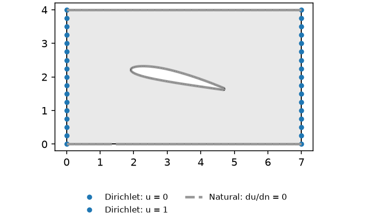
        'A potential difference across the channel (phi = 0 at the inlet, 1 at the '
        'outlet) drives the flow left to right; the walls and the wing surface take no '
        'condition, so no flow crosses them.',
        panel_aspect=1.8)


def demo(**kwargs) -> DemoResult:
    """Poisson's equation as potential flow over a NACA airfoil, on P2 elements."""
    s = run(**kwargs)
    return DemoResult([_flow_figure(s), _conditions_figure(s)])


# Builds its own airfoil-in-a-channel from the NACA formula, so it takes no domain.
DEMO = Demo('poisson', demo, section='Meshing & solving PDEs',
            show_source=physics,
            smoke_kwargs={'n_points': 40, 'max_area_fraction': 0.02})