outline_to_mesh

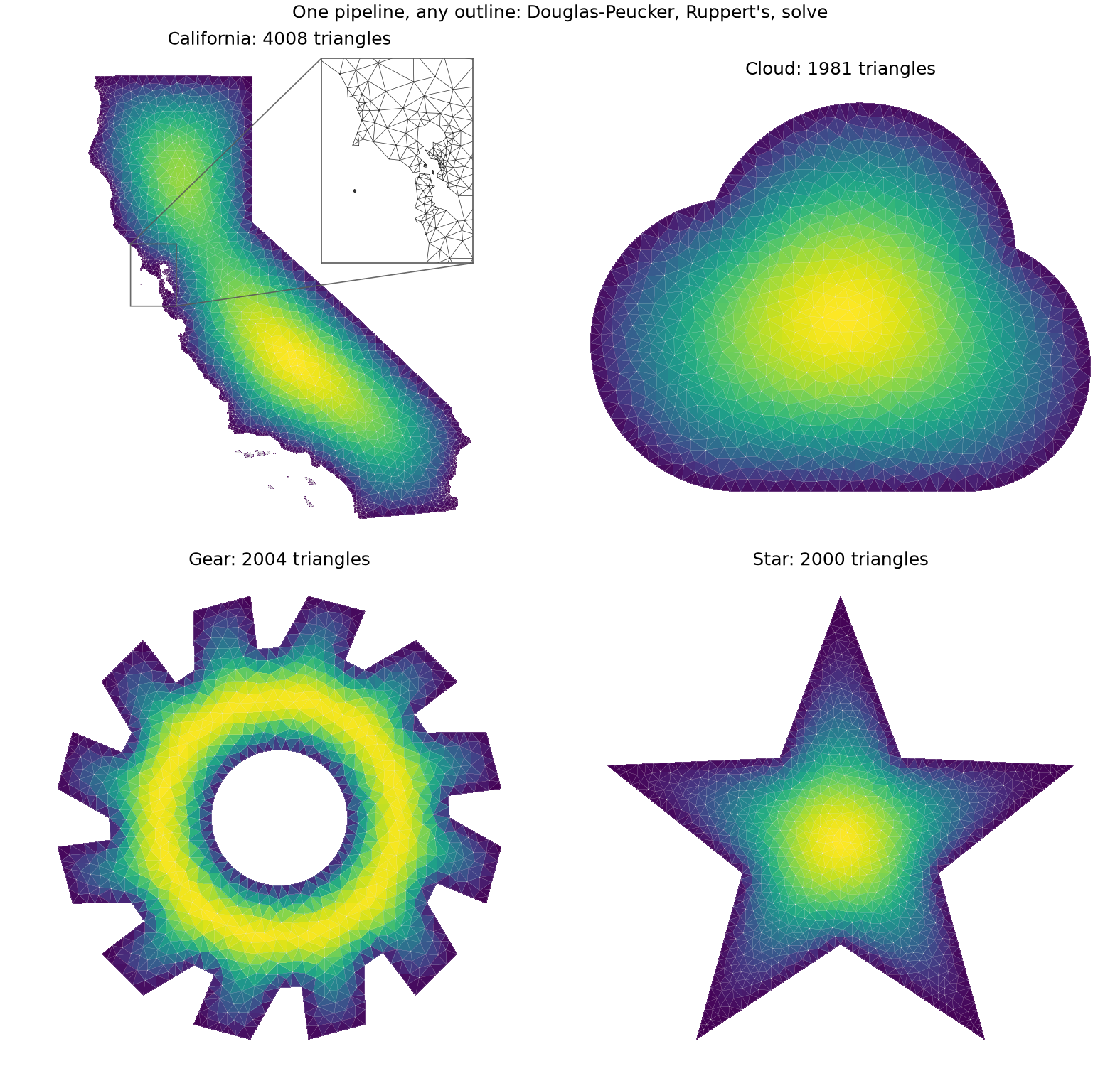
"""Four outlines, traced and generated, through one pipeline: simplify the traced
ones with Douglas-Peucker, triangulate with Ruppert's algorithm, and solve a Poisson
problem on each.

`zoo_shapes` gathers the outlines, `mesh_outline` and `dome` handle one each, and `run`
returns an `OutlineStudy` of plain results. Nothing here draws: `figures.py` does that
from the `OutlineStudy`, and this file is what the gallery shows.
"""
import json
from dataclasses import dataclass
from pathlib import Path

import numpy as np

from fem.boundary import Dirichlet
from fem.conditions import Conditions
from fem.loads import Source
from fem.mesh.curves import Circle
from fem.mesh.mesh import Mesh
from fem.mesh.outline import Outline, douglas_peucker
from fem.physics.equations import Poisson
from fem.regions import everywhere


def star_outline(points: int = 5, outer_radius: float = 1.0, inner_radius: float = 0.42,
                 center: tuple[float, float] = (0.0, 0.0)) -> Outline:
    """A `points`-pointed star as a single straight-line loop.

    Radii alternate between `outer_radius` at the tips and `inner_radius` at the notches,
    so the reentrant notches are the sharp corners Ruppert's meets at the input angle
    rather than refining away.
    """
    angles = np.pi / 2 + np.linspace(0, 2 * np.pi, 2 * points, endpoint=False)
    radii = np.where(np.arange(2 * points) % 2 == 0, outer_radius, inner_radius)
    outline = np.column_stack([center[0] + radii * np.cos(angles),
                               center[1] + radii * np.sin(angles)])
    return Outline.from_polygons([outline])


def gear_outline(teeth: int = 12, root_radius: float = 0.7, tooth_height: float = 0.22,
                 tooth_fraction: float = 0.5, bore_radius: float = 0.28,
                 center: tuple[float, float] = (0.0, 0.0)) -> Outline:
    """A spur gear with a circular bore, as two loops (rim and hole).

    Each of `teeth` sectors carries one tooth: the radius steps from `root_radius` out to
    `root_radius + tooth_height` over the middle `tooth_fraction` of the sector and back,
    with radial flanks. The bore is a `Circle`, so an isoparametric solve reads
    a true round hole and refinement rounds it; under the even-odd rule it is a hole in
    the gear rather than a second part.
    """
    tip_radius = root_radius + tooth_height
    pitch = 2 * np.pi / teeth
    gap = 0.5 * (1 - tooth_fraction) * pitch     # root arc either side of each tooth
    outline = []
    for i in range(teeth):
        base = i * pitch
        # (root, base) -> (root, base+gap): the valley; then radial flank up, the tip
        # land, and the next flank down is the following sector's opening edge.
        for radius, angle in ((root_radius, base), (root_radius, base + gap),
                              (tip_radius, base + gap), (tip_radius, base + pitch - gap)):
            outline.append((center[0] + radius * np.cos(angle),
                            center[1] + radius * np.sin(angle)))

    return Outline([Outline.from_polygons([np.array(outline)]).loops[0],
                    Circle(list(center), bore_radius)])

# Resolved against the repo, so a demo does not depend on where it was launched from.
DEFAULT_SVG_FILE = str(Path(__file__).resolve().parents[3] / 'files' / 'california.svg')
CLOUD_SVG_FILE = str(Path(__file__).resolve().parents[3] / 'files' / 'cloud.svg')

# Douglas-Peucker: drop points that deviate less than this fraction of the curve's
# bounding-box extent. Ruppert's cost grows steeply in point count.
DEFAULT_SIMPLIFICATION_TOLERANCE = 0.005

# The Poisson "dome": a unit source pinned to zero on every boundary, so the field is a
# picture of the domain itself, tallest where it is widest.
dome_bc = Conditions(Dirichlet(everywhere(), 0), Source(1.0))
dome_equation = Poisson()


def get_curve_from_svg(svg_file):
    """The longest loop of the SVG, as the ring of points its pieces sample to."""
    longest = max(Outline.from_svg(svg_file).loops, key=len)
    return Outline([longest]).sample().vertices


def close_ring(points):
    """`points` with its first vertex repeated at the end, for plotting.

    A closed SVG path comes back as a ring whose closing edge is implied;
    `ax.plot` needs it spelled out.
    """
    return np.vstack([points, points[:1]])


def curve_extent(curve) -> float:
    """The longer side of `curve`'s bounding box, which the tolerance is a fraction of."""
    return float(max(np.max(curve, axis=0) - np.min(curve, axis=0)))


def simplify_curve(curve, tolerance=DEFAULT_SIMPLIFICATION_TOLERANCE):
    """Simplify `curve` with Douglas-Peucker, `tolerance` a fraction of its extent."""
    return douglas_peucker(curve, tolerance * curve_extent(curve))


def save_curve(curve, save_file='douglas_peucker_output.json'):
    """Write a simplified curve out as JSON, to be read back as an outline later."""
    with open(save_file, 'w') as f:
        json.dump(np.asarray(curve).tolist(), f)


def zoo_shapes(svg_tolerance=DEFAULT_SIMPLIFICATION_TOLERANCE) -> list[tuple[str, Outline]]:
    """The outlines the zoo meshes, as (name, Outline) pairs.

    California and the cloud are traced from `files/*.svg` and simplified on the way in;
    the star and gear are generated (below). Each puts a different demand on the
    mesher: disconnected islands, a curved boundary, sharp reentrant corners, and
    repeated teeth around a circular bore.
    """
    return [
        ('California', Outline.from_svg(DEFAULT_SVG_FILE).simplified(svg_tolerance)),
        ('Cloud', Outline.from_svg(CLOUD_SVG_FILE).simplified(svg_tolerance)),
        ('Gear', gear_outline()),
        ('Star', star_outline()),
    ]


def dome(mesh: Mesh) -> np.ndarray:
    """Solve -div(grad u) = 1 with u = 0 on every boundary of `mesh`."""
    return dome_equation.problem(mesh, dome_bc).solve().dofs


@dataclass
class MeshedOutline:
    """One outline through the pipeline: its name, point count, mesh, and dome."""
    name: str
    n_points: int
    mesh: Mesh
    dofs: np.ndarray

    @property
    def n_triangles(self) -> int:
        return len(self.mesh.elements)

    @property
    def worst_angle(self) -> float:
        """The smallest angle in the mesh (degrees), against the bound Ruppert's was set."""
        return self.mesh.min_angle


@dataclass
class OutlineStudy:
    """Everything `run` computed, for the figure and the table to read."""
    shapes: list[MeshedOutline]
    min_angle: float


def run(min_angle=28, max_area_fraction=0.0008, svg_tolerance=0.001) -> OutlineStudy:
    """Mesh and solve every outline in the zoo.

    `svg_tolerance` is finer than the default so the coastline keeps its detail (the
    raw trace has ~1700 points).
    """
    shapes = []
    for name, outline in zoo_shapes(svg_tolerance):
        graph = outline.sample()
        mesh = graph.mesh(min_angle=min_angle, max_area_fraction=max_area_fraction)
        shapes.append(MeshedOutline(name, len(graph.vertices), mesh, dome(mesh)))
    return OutlineStudy(shapes, min_angle)