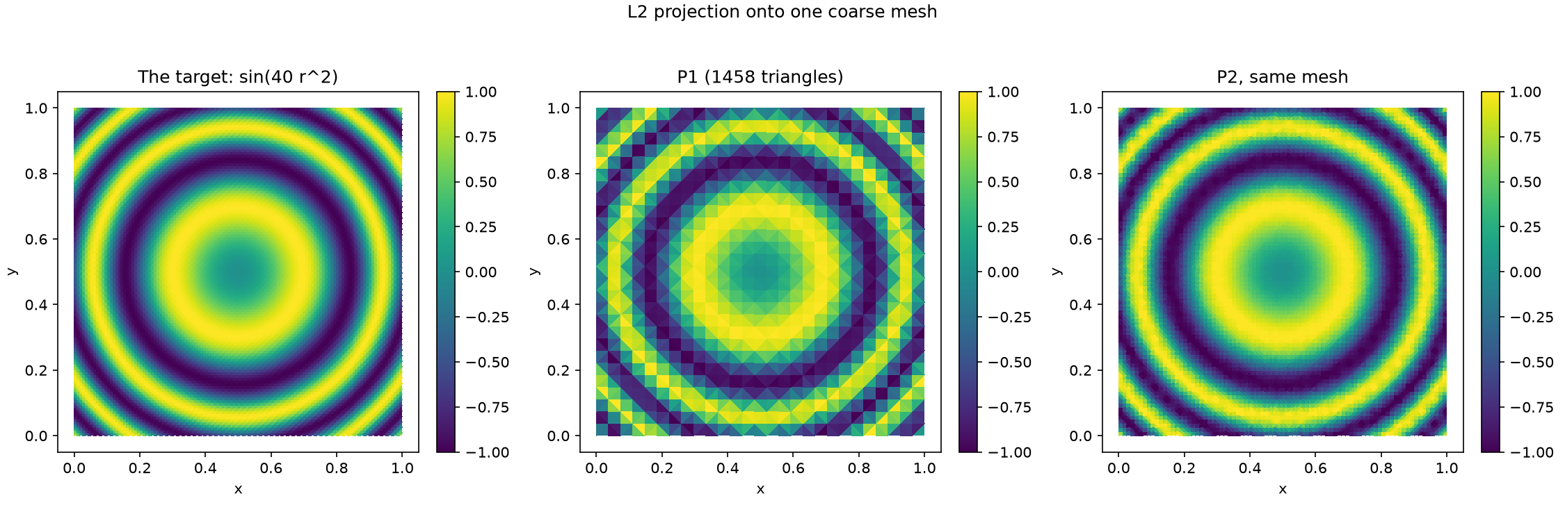
An oscillatory function projected onto a coarse mesh's P1 and P2 spaces, showing what each can represent.
uv run python examples/cli.py run l2_projection
The functions that pose and solve the problem. The figures are below the fold.
"""An oscillatory function projected onto one coarse mesh's P1 and P2 spaces.

`project` states and solves one projection; `run` returns a `ProjectionStudy` of plain
results. Nothing here draws: `figures.py` does that from the study, and this file is
what the gallery shows.
"""
from dataclasses import dataclass

import numpy as np

from fem.conditions import Conditions
from fem.elements import QuadraticTriangleElement
from fem.loads import Source
from fem.mesh.mesh import Mesh
from fem.physics.equations import Projection
from fem.post.solution import FieldSolution


def target(point):
    """sin(40 r^2) about the unit square's centre: rings that tighten with radius."""
    x, y = (point - np.array([0.5, 0.5])).T
    return [np.sin(40 * (x**2 + y**2))]


def project(mesh, element_type=None) -> FieldSolution:
    """The L2 projection of `target` onto the mesh's space of the given element."""
    return Projection().problem(mesh, Conditions(Source(target)), element_type=element_type).solve()


@dataclass
class ProjectionStudy:
    """Everything `run` computed, for the figure to read."""
    mesh: Mesh
    p1: FieldSolution
    p2: FieldSolution


def run(mesh) -> ProjectionStudy:
    """Project the target onto the mesh's P1 and P2 spaces."""
    return ProjectionStudy(mesh, project(mesh), project(mesh, QuadraticTriangleElement))
"""The figure of the L2 projection demo, drawn from a `ProjectionStudy`."""
from functools import partial

import numpy as np
from demo_registry import Demo, DemoResult, Figure

from demos.l2_projection import physics
from demos.l2_projection.physics import ProjectionStudy, run
from fem.mesh.structured import box_mesh
from fem.plot.plotter import Plotter


def _projection_figure(s: ProjectionStudy, reference_resolution) -> Figure:
    # The target sampled on a fine mesh, so the left panel is the function itself rather
    # than another coarse approximation of it. The projection (right) is on the demo's own
    # mesh, coarse enough that the fast outer rings outrun what P1 can represent.
    fine = box_mesh([[0.0, 0.0], [1.0, 1.0]], (reference_resolution, reference_resolution))
    xy = fine.vertices - np.array([0.5, 0.5])
    exact = np.sin(40 * (xy[:, 0]**2 + xy[:, 1]**2))

    plotter = Plotter(1, 3, title='L2 projection onto one coarse mesh')
    plotter.plot(fine, exact, mode='colored', idx=(0, 0), label='', clim=(-1, 1),
                 title='The target: sin(40 r^2)')
    plotter.plot(s.mesh, s.p1.dofs, mode='colored', idx=(0, 1), label='', clim=(-1, 1),
                 title=f'P1 ({len(s.mesh.elements)} triangles)')
    plotter.plot(s.mesh, s.p2.dofs, mode='colored', idx=(0, 2), label='', clim=(-1, 1),
                 title='P2, same mesh', space=s.p2.space)
    return Figure(
        plotter,
        'How well a space can represent a function at all, before any PDE. Left: the '
        'target sin(40 r^2), whose rings tighten with radius. Middle: its L2 projection '
        'onto the P1 space of a coarse mesh. The slow inner rings come through; where one '
        'ring spans only a couple of triangles the space can no longer follow it, and the '
        'outer rings break up into the mesh. Right: the P2 space of the same mesh, whose '
        'edge-midpoint nodes let each element curve, follows the rings further out. This '
        'representation error is the floor every solver on the mesh starts from.')


def demo(mesh, reference_resolution=120) -> DemoResult:
    """An oscillatory function projected onto a coarse mesh's P1 and P2 spaces, showing
    what each can represent."""
    s = run(mesh)
    return DemoResult([_projection_figure(s, reference_resolution)])


# Meshed coarse, so sin(40 r^2)'s slow inner rings resolve but the fast
# outer ones alias into the triangulation.
DEMO = Demo('l2_projection', demo, section='Accuracy & performance',
            domain=partial(box_mesh, [[0.0, 0.0], [1.0, 1.0]], (28, 28)), smoke_kwargs={'reference_resolution': 60},
            show_source=physics)