One clamped block stretched by a linear solve, by energy minimisation, and by two finite-strain material laws; then the same stretch walked up from zero, so the force-stretch curve separates the laws quantitatively.
uv run python examples/cli.py run elasticity_models
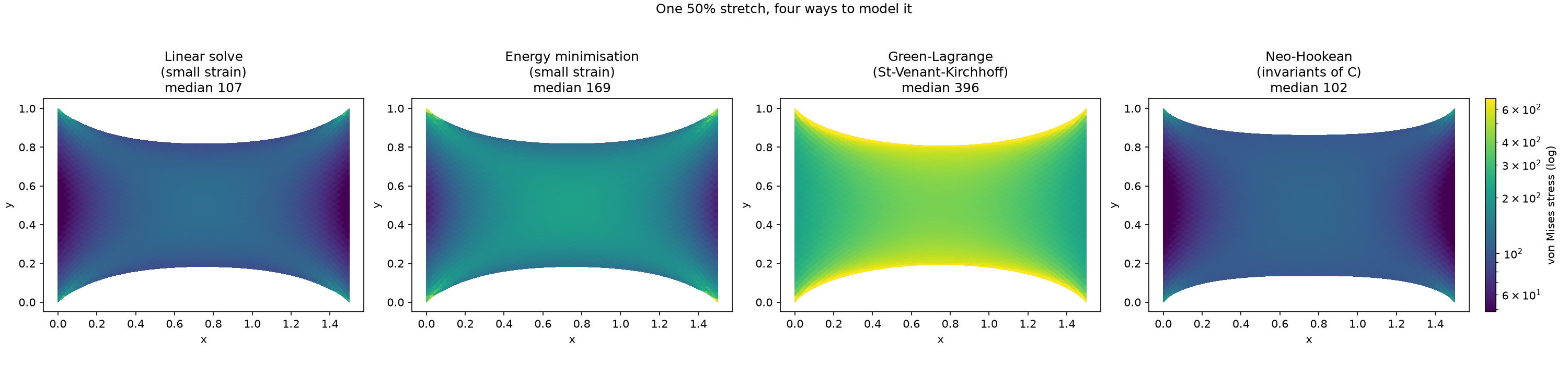
Panels 1 and 2 are the same physics, small-strain linear elasticity, solved two ways: panel 1 as a direct linear solve (K u = f), panel 2 by minimising the elastic energy with Newton. They reach the same displacement to machine precision, so the colour difference is not a physics difference. Panel 1 reports engineering stress sigma = D:eps, force per unit original area; panel 2 reports true (Cauchy) stress, force per unit deformed area. Because stretching thins the cross-section, the same internal force reads higher as true stress, about 50% higher here, near the 1.5 stretch factor. The two coincide only at small strain, when the geometry barely moves.
Panels 2, 3 and 4 hold the method fixed and change the material. Panel 2 is small strain; panels 3 and 4 are nonlinear, finite-strain elasticity. St-Venant-Kirchhoff (panel 3) is the simplest finite-strain model, small-strain elasticity rewritten on the Green-Lagrange strain. Its strength is that it is frame-indifferent, a rigid rotation stores no energy, which small strain gets wrong; its weakness is that its energy is polynomial in the stretch, so it over-stiffens steeply in tension and loses stability in strong compression. In the plot it is by far the most stressed panel (median 396, several times the interior stress of the others), the block lit up and fighting the stretch.
Neo-Hookean (panel 4) is a rubber-elasticity model written in the invariants of C = F^T F with a ln J volumetric term. Its strength is a physically realistic large-strain response, it does not over-stiffen in tension and stays stable in compression and near incompressibility; its cost is a more expensive, non-polynomial evaluation that must guard against element inversion. In the plot it is the calmest finite-strain panel, moderate stress everywhere, its median (102) sitting right next to the linear baseline (107).
displacement, linear solve vs energy minimisation: relative difference 3.3e-14
minimised elastic energy: 33.63
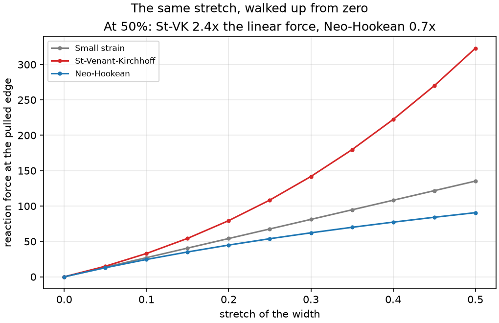
reaction at 50% stretch (vs small strain): St-Venant-Kirchhoff 2.39x, Neo-Hookean 0.67x
The functions that pose and solve the problem. The figures are below the fold.
"""One clamped block stretched four ways: a linear solve, energy minimisation, and two
finite-strain material laws — then the same stretch walked up from zero, so the
force-stretch curve separates the laws quantitatively.

`stretch_bc` states the condition and `stretch_four_ways` solves it;
`load_deflection` ramps the stretch through `QuasiStaticStepping` and reads the
reaction force at every level. `run` calls them and returns a `StretchStudy` of plain
results. Nothing here draws: `figures.py` does that from the `StretchStudy`, and this
file is what the gallery shows.
"""
from dataclasses import dataclass

import numpy as np

from fem.algebra.solve import BacktrackingLineSearch, NewtonSolve
from fem.algebra.stepping import QuasiStaticStepping
from fem.boundary import Dirichlet
from fem.conditions import Conditions, Initial
from fem.mesh.mesh import Mesh
from fem.mesh.structured import box_mesh
from fem.physics.energies import NeohookeanEnergyDensity
from fem.physics.equations import FiniteStrainElastic, LinearElastic
from fem.physics.forms import EnergyForm
from fem.post.solution import ElasticSolution
from fem.problem import Problem
from fem.regions import on_plane

E, NU = 200.0, 0.4


def stretch_bc(width, stretch) -> Conditions:
    """Both ends Dirichlet: the left held at zero, the right displaced to `stretch` of
    the width. Nothing is loaded."""
    return Conditions(
        Dirichlet(on_plane(0, 0.0), [0, 0]),
        Dirichlet(on_plane(0, width), [stretch*width, 0]),
    )


def stretch_four_ways(mesh: Mesh, bc: Conditions):
    """Solve the stretch as a linear system, as an energy minimisation, and under the
    St-Venant-Kirchhoff and Neo-Hookean finite-strain laws.

    The first two are the same physics reached two ways: solving K u = f, and Newton
    on the elastic energy that system is the stationary point of. Their displacements
    agree to machine precision. Their stress does not, since the two recover different
    measures: sigma = D:eps against the true Cauchy stress J^-1 P F^T at the deformed
    configuration, which agree only to O(||grad u||).

    The last two change the physics: two finite-strain laws that share the same
    small-strain linearisation but differ once the stretch is large. Green-Lagrange
    St-Venant-Kirchhoff has a polynomial energy; Neo-Hookean is written in the
    invariants of C = F^T F and carries the log J terms that keep it stable in
    compression. Both reach the same energy at small strain and part company here.

    The finite-strain solves are seeded with the linear solution. Seeded from zero,
    the elements beside the displaced edge start stretched by the whole prescribed
    displacement over one element width, and Newton's early steps from there teeter on
    inverting them (a J <= 0 element has infinite Neo-Hookean energy); the small-strain
    answer is a few Newton steps from either finite-strain one.

    Returns the named solutions, and the energy problem with its minimiser.
    """
    linear = LinearElastic(E=E, nu=NU)
    stvk = FiniteStrainElastic(E=E, nu=NU)
    neohookean = FiniteStrainElastic(E=E, nu=NU, law=NeohookeanEnergyDensity)
    # The second solve states small strain as an energy and minimises it: the same
    # density the linear stiffness is the Hessian of, under Newton.
    energy_problem = Problem(linear.space(mesh), EnergyForm(linear.energy_density()), bc)
    energy_u = NewtonSolve(line_search=BacktrackingLineSearch()).solve(energy_problem)
    linear_solution = linear.problem(mesh, bc).solve()
    newton = NewtonSolve(line_search=BacktrackingLineSearch())
    solutions = [
        ('Linear solve\n(small strain)', linear_solution),
        ('Energy minimisation\n(small strain)', energy_problem.solution(energy_u)),
        ('Green-Lagrange\n(St-Venant-Kirchhoff)',
         stvk.problem(mesh, bc).solve(strategy=newton, initial=Initial(linear_solution))),
        ('Neo-Hookean\n(invariants of C)',
         neohookean.problem(mesh, bc).solve(strategy=newton, initial=Initial(linear_solution))),
    ]
    return solutions, energy_problem, energy_u


def load_deflection(width, stretch, steps=10, resolution=24):
    """Walk the stretch up from zero and read the force it takes, per material law.

    The pulled edge is displacement-controlled, so the load is the reaction: the
    internal force at that edge's x DOFs, summed. `QuasiStaticStepping` scales the
    prescribed displacement to each level and warm-starts Newton from the last one,
    which is also how a finite-strain solve is walked past a seed a single solve
    would diverge from. A coarse mesh of its own: the curve is a global scalar per
    level, converged long before the stress field of the main figure is.

    Returns `[(name, stretches, forces)]`, one triple per law.
    """
    mesh = box_mesh([[0.0, 0.0], [width, width]], (resolution, resolution))
    bc = stretch_bc(width, stretch)
    models = [
        ('Small strain', LinearElastic(E=E, nu=NU)),
        ('St-Venant-Kirchhoff', FiniteStrainElastic(E=E, nu=NU)),
        ('Neo-Hookean', FiniteStrainElastic(E=E, nu=NU, law=NeohookeanEnergyDensity)),
    ]
    stepping = QuasiStaticStepping(steps=steps)
    curves = []
    for name, equation in models:
        problem = equation.problem(mesh, bc)
        history = stepping.solve(problem)
        pulled = np.isclose(problem.space.node_coords[:, 0], width)
        x_dofs = 2 * np.flatnonzero(pulled)
        forces = np.array([float(problem.internal_residual(u)[x_dofs].sum())
                           for u in history.dofs])
        curves.append((name, history.t * stretch, forces))
    return curves


@dataclass
class StretchStudy:
    """Everything `run` computed, for the figures and the summary to read."""
    mesh: Mesh
    stretch: float
    bc: Conditions
    solutions: list[tuple[str, ElasticSolution]]   # (panel name, solution)
    energy_problem: Problem
    energy_u: np.ndarray
    curves: list[tuple[str, np.ndarray, np.ndarray]]   # (law, stretches, reaction forces)

    @property
    def von_mises(self) -> list[np.ndarray]:
        return [solution.von_mises for _, solution in self.solutions]

    @property
    def drift(self) -> float:
        """Relative difference between the linear and energy-minimised displacements."""
        linear_u = self.solutions[0][1].dofs
        return float(np.linalg.norm(self.energy_u - linear_u) / np.linalg.norm(linear_u))

    @property
    def minimised_energy(self) -> float:
        return float(self.energy_problem.energy(self.energy_u))


def run(mesh: Mesh, stretch=0.5, curve_steps=10, curve_resolution=24) -> StretchStudy:
    """Stretch the block on `mesh` by `stretch` of its width, four ways; then walk the
    same stretch up from zero for the force-stretch curve of each law."""
    width = np.max(mesh.vertices[:, 0])
    bc = stretch_bc(width, stretch)
    solutions, energy_problem, energy_u = stretch_four_ways(mesh, bc)
    curves = load_deflection(width, stretch, curve_steps, curve_resolution)
    return StretchStudy(mesh, stretch, bc, solutions, energy_problem, energy_u, curves)
"""The figures and summary of the elasticity models demo, drawn from a `StretchStudy`."""
from functools import partial

import numpy as np
from demo_registry import Demo, DemoResult, Figure

from demos._charts import conditions_figure
from demos.elasticity_models import physics
from demos.elasticity_models.physics import StretchStudy, run
from fem.mesh.structured import box_mesh
from fem.plot.plotter import Plotter


def _stress_figure(s: StretchStudy) -> Figure:
    # The four fields span roughly a factor of ten (Neo-Hookean's interior against
    # St-VK's), so one shared *log* colour scale carries them all: each panel keeps its
    # own structure while magnitudes still compare across panels. The stress diverges at
    # the clamped corners, where the imposed displacement is singular (it grows without
    # bound under refinement, a mesh artefact, not a material fact), so the scale is
    # capped at the 99th percentile of the pooled field, those corner nodes saturate, and
    # the per-panel median is the exact number.
    vms = s.von_mises
    pooled = np.concatenate([np.ravel(v) for v in vms])
    # A positive floor (log needs one) and a cap that drops the singular corners, both
    # from the pooled field so the four scales are identical.
    lo = float(np.percentile(pooled[pooled > 0], 1))
    hi = float(np.percentile(pooled, 99))

    plotter = Plotter(1, 4, title=f'One {s.stretch:.0%} stretch, four ways to model it')
    for i, ((name, solution), vm) in enumerate(zip(s.solutions, vms, strict=True)):
        plotter.plot(solution.deformed_mesh(), vm, mode='colored', idx=(0, i),
                     label='von Mises stress (log)', clim=(lo, hi), log_scale=True,
                     colorbar=(i == len(s.solutions) - 1),
                     title=f'{name}\nmedian {np.median(vm):.0f}')
    return Figure(
        plotter,
        'Four solves of one boundary condition: the left edge clamped, the right edge '
        'pulled to a 50% stretch, nothing else loaded. One shared log colour scale '
        'spans all four panels, so magnitudes compare directly across them; the median '
        'under each title is the exact figure, and the singular clamped corners '
        'saturate at the top.',
        'stress',
        body=[
            'Panels 1 and 2 are the same physics, small-strain linear elasticity, '
            'solved two ways: panel 1 as a direct linear solve (K u = f), panel 2 by '
            'minimising the elastic energy with Newton. They reach the same '
            'displacement to machine precision, so the colour difference is not a '
            'physics difference. Panel 1 reports engineering stress sigma = D:eps, '
            'force per unit original area; panel 2 reports true (Cauchy) stress, force '
            'per unit deformed area. Because stretching thins the cross-section, the '
            'same internal force reads higher as true stress, about 50% higher here, '
            'near the 1.5 stretch factor. The two coincide only at small strain, when '
            'the geometry barely moves.',

            'Panels 2, 3 and 4 hold the method fixed and change the material. Panel 2 '
            'is small strain; panels 3 and 4 are nonlinear, finite-strain elasticity. '
            'St-Venant-Kirchhoff (panel 3) is the simplest finite-strain model, '
            'small-strain elasticity rewritten on the Green-Lagrange strain. Its '
            'strength is that it is frame-indifferent, a rigid rotation stores no '
            'energy, which small strain gets wrong; its weakness is that its energy is '
            'polynomial in the stretch, so it over-stiffens steeply in tension and '
            'loses stability in strong compression. In the plot it is by far the most '
            'stressed panel (median 396, several times the interior stress of the '
            'others), the block lit up and fighting the stretch.',

            'Neo-Hookean (panel 4) is a rubber-elasticity model written in the '
            'invariants of C = F^T F with a ln J volumetric term. Its strength is a '
            'physically realistic large-strain response, it does not over-stiffen in '
            'tension and stays stable in compression and near incompressibility; its '
            'cost is a more expensive, non-polynomial evaluation that must guard '
            'against element inversion. In the plot it is the calmest finite-strain '
            'panel, moderate stress everywhere, its median (102) sitting right next to '
            'the linear baseline (107).',
        ])


def _force_figure(s: StretchStudy) -> Figure:
    # The stress panels show one endpoint; this walks the whole path there. Each curve
    # is the reaction force the pulled edge takes at every level of the stretch,
    # solved by quasi-static stepping (each level's solve seeded with the last).
    figure = Plotter(1, 1, figsize=(6.8, 4.4),
                     title='The same stretch, walked up from zero')
    ax = figure.chart_ax(idx=(0, 0), xlabel='stretch of the width',
                         ylabel='reaction force at the pulled edge')
    colors = {'Small strain': 'tab:gray', 'St-Venant-Kirchhoff': 'tab:red',
              'Neo-Hookean': 'tab:blue'}
    for name, stretches, forces in s.curves:
        ax.plot(stretches, forces, 'o-', markersize=3, color=colors[name], label=name)
    ax.grid(alpha=0.3)
    ax.legend(loc='upper left', fontsize='small')

    end = {name: forces[-1] for name, _, forces in s.curves}
    stvk = end['St-Venant-Kirchhoff'] / end['Small strain']
    neo = end['Neo-Hookean'] / end['Small strain']
    ax.set_title(f'At {s.stretch:.0%}: St-VK {stvk:.1f}x the linear force, '
                 f'Neo-Hookean {neo:.1f}x')
    return Figure(
        figure,
        f'The force it takes to hold each level of the stretch, from rest to '
        f'{s.stretch:.0%}, one curve per material law. Small strain is a straight '
        f'line by construction. St-Venant-Kirchhoff bends upward, its polynomial '
        f'energy over-stiffening until the final level costs {stvk:.1f}x the linear '
        f'force; Neo-Hookean bends downward to {neo:.1f}x, the section thinning '
        f'faster than the law stiffens. The endpoint panels above show only where '
        f'these curves end; the walk itself is quasi-static stepping, each level '
        f'solved with the previous one as the seed.',
        'force')


def _conditions_figure(s: StretchStudy) -> Figure:
    return conditions_figure(
        s.mesh, s.bc,
        'Both ends are Dirichlet. The left is held at zero and the right is displaced '
        f'to {s.stretch:.0%} of the width. Nothing is loaded; the stress above is what '
        'it costs to hold that shape.')


def _summary(s: StretchStudy) -> str:
    end = {name: forces[-1] for name, _, forces in s.curves}
    return (f'displacement, linear solve vs energy minimisation: '
            f'relative difference {s.drift:.1e}\n'
            f'minimised elastic energy: {s.minimised_energy:.4g}\n'
            f'reaction at {s.stretch:.0%} stretch (vs small strain): '
            f'St-Venant-Kirchhoff {end["St-Venant-Kirchhoff"] / end["Small strain"]:.2f}x, '
            f'Neo-Hookean {end["Neo-Hookean"] / end["Small strain"]:.2f}x')


def demo(mesh, **kwargs) -> DemoResult:
    """One clamped block stretched by a linear solve, by energy minimisation, and by two
    finite-strain material laws; then the same stretch walked up from zero, so the
    force-stretch curve separates the laws quantitatively."""
    s = run(mesh, **kwargs)
    return DemoResult([_stress_figure(s), _force_figure(s), _conditions_figure(s)],
                      text=_summary(s))


# A square keeps the deformed and undeformed shapes comparable at a glance.
DEMO = Demo('elasticity_models', demo, section='Solids & structures',
            domain=partial(box_mesh, [[0.0, 0.0], [1.0, 1.0]], (60, 60)),
            smoke_kwargs={'curve_steps': 3, 'curve_resolution': 8}, show_source=physics)