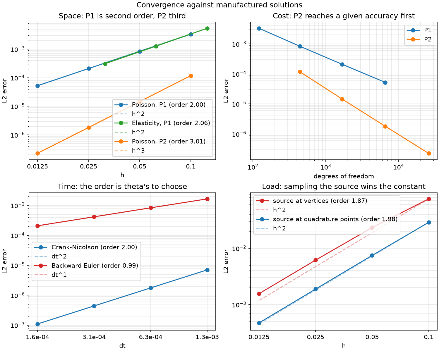
Convergence rates in space and time against manufactured solutions, P1 against P2, and the load built two ways.
uv run python examples/cli.py run convergence
                      fitted order   expected
Poisson P1 (h)             2.00          2
Poisson P2 (h)             3.01          3
Poisson 3D (h)             1.95          2
Elasticity (h)             2.06          2
Neumann/Robin (h)          2.00          2
Crank-Nicolson (dt)        2.00          2
Backward Euler (dt)        0.99          1
Nodal load (h)             1.87          2
Sampled load (h)           1.98          2
The functions that pose and solve the problem. The figures are below the fold.
"""Convergence rates in space and time against manufactured solutions.

The one demo that shows not what the solver computed but how wrong it was:

  in space  P1 elements are O(h^2) (halve h, quarter the error) for a scalar
            unknown and for a coupled vector one alike; P2 is O(h^3);
  in time   the theta method's order is theta's to choose: 1 at backward Euler,
            2 at Crank-Nicolson, the default.

The same studies run as assertions in tests/test_convergence.py and tests/test_convergence_heat.py.
`run` gathers them into a `RatesStudy` of plain results. Nothing here draws:
`figures.py` does that from the study, and this file is what the gallery shows.
"""
from dataclasses import dataclass

import numpy as np
from mms import (
    ConvergenceStudy,
    elastic_convergence,
    load_comparison_convergence,
    mixed_bc_convergence,
    poisson_convergence,
    poisson_p2_convergence,
    theta_convergence,
)

from fem.elements import QuadraticTriangleElement
from fem.space import FunctionSpace


def space_studies(resolutions, elastic_resolutions):
    """P1 and P2 Poisson and P1 elasticity against h, with the DOF counts of the two
    Poisson sequences for the accuracy-per-cost view: P2 spends more unknowns per
    element, and the question is whether its faster rate pays that back."""
    solves = poisson_convergence(resolutions)
    p2_solves = poisson_p2_convergence(resolutions)
    p1_dofs = np.array([FunctionSpace(s.mesh).n_dofs for s in solves])
    p2_dofs = np.array([FunctionSpace(s.mesh, QuadraticTriangleElement).n_dofs
                        for s in p2_solves])
    return (ConvergenceStudy.from_solves(solves), ConvergenceStudy.from_solves(p2_solves),
            ConvergenceStudy.from_solves(elastic_convergence(elastic_resolutions)),
            p1_dofs, p2_dofs)


def time_studies(step_counts):
    """Crank-Nicolson and backward Euler against dt.

    Step counts chosen to sit in the asymptotic band: over coarser steps Crank-Nicolson
    reads an order near 3, because lambda*dt is not yet small and the leading error term
    is not yet the one that dominates.
    """
    return theta_convergence(0.5, step_counts), theta_convergence(1.0, step_counts)


def load_studies(resolutions):
    """The same P1 solve with the source read only at the vertices (its linear
    interpolant) against one sampled at the quadrature points: the rate is the same,
    the constant is not."""
    loads = load_comparison_convergence(resolutions)
    steps = np.array([lc.h for lc in loads])
    nodal = ConvergenceStudy(steps, np.array([lc.nodal_error for lc in loads]))
    sampled = ConvergenceStudy(steps, np.array([lc.sampled_error for lc in loads]))
    return nodal, sampled


@dataclass
class RatesStudy:
    """Everything `run` computed, for the figure and the table to read."""
    poisson: ConvergenceStudy
    p2: ConvergenceStudy
    elastic: ConvergenceStudy
    p1_dofs: np.ndarray
    p2_dofs: np.ndarray
    crank_nicolson: ConvergenceStudy
    backward_euler: ConvergenceStudy
    nodal: ConvergenceStudy
    sampled: ConvergenceStudy
    poisson_3d: ConvergenceStudy
    mixed_bc: ConvergenceStudy

    @property
    def table(self) -> list[tuple[str, ConvergenceStudy, int]]:
        """Each study with its name and the order theory expects of it."""
        return [('Poisson P1 (h)', self.poisson, 2),
                ('Poisson P2 (h)', self.p2, 3),
                ('Poisson 3D (h)', self.poisson_3d, 2),
                ('Elasticity (h)', self.elastic, 2),
                ('Neumann/Robin (h)', self.mixed_bc, 2),
                ('Crank-Nicolson (dt)', self.crank_nicolson, 2),
                ('Backward Euler (dt)', self.backward_euler, 1),
                ('Nodal load (h)', self.nodal, 2),
                ('Sampled load (h)', self.sampled, 2)]


def run(resolutions=(11, 21, 41, 81), elastic_resolutions=(9, 17, 33),
        step_counts=(16, 32, 64, 128), poisson_3d_resolutions=(5, 9, 13)) -> RatesStudy:
    """Run every study and collect the measured rates."""
    poisson, p2, elastic, p1_dofs, p2_dofs = space_studies(resolutions, elastic_resolutions)
    crank_nicolson, backward_euler = time_studies(step_counts)
    nodal, sampled = load_studies(resolutions)
    poisson_3d = ConvergenceStudy.from_solves(poisson_convergence(poisson_3d_resolutions, dim=3))
    mixed_bc = ConvergenceStudy.from_solves(mixed_bc_convergence(resolutions))
    return RatesStudy(poisson, p2, elastic, p1_dofs, p2_dofs, crank_nicolson, backward_euler,
                      nodal, sampled, poisson_3d, mixed_bc)
"""The figure and table of the convergence demo, drawn from a `RatesStudy`."""
from demo_registry import Demo, DemoResult, Figure

from demos._charts import tidy_log_axis
from demos.convergence import physics
from demos.convergence.physics import RatesStudy, run
from fem.plot.plotter import Plotter


def _plot_study(ax, study, label, colour, reference_order, xlabel):
    """One measured curve plus the power law it is being held to."""
    ax.loglog(study.step, study.error, 'o-', color=colour,
              label=f'{label} (order {study.fitted_order:.2f})')
    # Anchored at the coarsest point, so the two lines start together and any gap is
    # the measured rate differing from the reference rather than an offset between them.
    reference = study.error[0] * (study.step / study.step[0])**reference_order
    ax.loglog(study.step, reference, '--', color=colour, alpha=0.4,
              label=f'{xlabel}^{reference_order}')


def _rates_figure(s: RatesStudy) -> Figure:
    plotter = Plotter(2, 2, figsize=(10.0, 8.0),
                      title='Convergence against manufactured solutions')
    space = plotter.chart_ax(idx=(0, 0), xlabel='h', ylabel='L2 error')
    _plot_study(space, s.poisson, 'Poisson, P1', 'tab:blue', 2, 'h')
    _plot_study(space, s.elastic, 'Elasticity, P1', 'tab:green', 2, 'h')
    _plot_study(space, s.p2, 'Poisson, P2', 'tab:orange', 3, 'h')
    space.set_title('Space: P1 is second order, P2 third')
    tidy_log_axis(space, s.poisson.step)

    cost = plotter.chart_ax(idx=(0, 1), xlabel='degrees of freedom', ylabel='L2 error')
    cost.loglog(s.p1_dofs, s.poisson.error, 'o-', color='tab:blue', label='P1')
    cost.loglog(s.p2_dofs, s.p2.error, 'o-', color='tab:orange', label='P2')
    cost.set_title('Cost: P2 reaches a given accuracy first')
    cost.grid(True, which='both', alpha=0.3)
    cost.legend()

    time = plotter.chart_ax(idx=(1, 0), xlabel='dt', ylabel='L2 error')
    _plot_study(time, s.crank_nicolson, 'Crank-Nicolson', 'tab:blue', 2, 'dt')
    _plot_study(time, s.backward_euler, 'Backward Euler', 'tab:red', 1, 'dt')
    time.set_title("Time: the order is theta's to choose")
    tidy_log_axis(time, s.crank_nicolson.step)

    load = plotter.chart_ax(idx=(1, 1), xlabel='h', ylabel='L2 error')
    _plot_study(load, s.nodal, 'source at vertices', 'tab:red', 2, 'h')
    _plot_study(load, s.sampled, 'source at quadrature points', 'tab:blue', 2, 'h')
    load.set_title('Load: sampling the source wins the constant')
    tidy_log_axis(load, s.nodal.step)
    return Figure(
        plotter,
        'Top left: on the same meshes, halving h quarters the P1 error (order 2), '
        'for a scalar unknown and for a coupled vector one alike, and divides the P2 '
        'error by eight (order 3). Top right: the same errors against the number of '
        'unknowns; P2 spends more DOFs per element but reaches a given accuracy with '
        'fewer of them. Bottom left: the error against the time step, where backward '
        'Euler is first order and Crank-Nicolson second, for the same cost per step. '
        'Bottom right: an oscillatory source read only at the vertices against one '
        'sampled at the quadrature points. Both are second order; the sampled load '
        'is about 3x more accurate on every mesh.')


def _summary(s: RatesStudy) -> str:
    rows = ['                      fitted order   expected']
    for name, study, expected in s.table:
        rows.append(f'{name:<22}{study.fitted_order:>9.2f}{expected:>11}')
    return '\n'.join(rows)


def demo(**kwargs) -> DemoResult:
    """Convergence rates in space and time against manufactured solutions, P1 against
    P2, and the load built two ways."""
    s = run(**kwargs)
    return DemoResult([_rates_figure(s)], text=_summary(s))


# Builds its own refinement sequence; the smoke run keeps the two coarsest meshes.
DEMO = Demo('convergence', demo, section='Accuracy & performance',
            smoke_kwargs={'resolutions': (11, 21), 'elastic_resolutions': (9, 17),
                          'step_counts': (16, 32), 'poisson_3d_resolutions': (5, 9)},
            show_source=physics)